Introduction to Excel
Sorting Data, AutoFilter and Freeze panes
Download Sorting Data pdf :Autofilter and freeze panes
You can use sorting to organise your spreadsheet data in ascending or descending order. You are allowed upto three levels of sort for example, if you sort by Surname in ascending order and then First name in ascending order, when Excel comes across two people called “smith”, it would then put them in first name order “Colin” and then “Robert” for example.
- Move to a cell in the column you want to sort by.
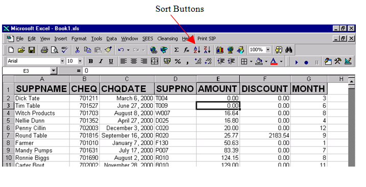
- Click on the Sort Ascending button to sort A-Z, 1-100 or
- Click on the Sort Descending button to sort Z-A, 100-1
To Sort data using up to three fields
- Move to a cell inside your data
- Click on the Data menu, and then click on the sort command
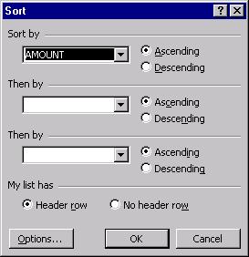
- The Sort dialogue box will be displayed.
- If your list has text field names, click on the header Row option under the My list has command, if Excel has not selected it automatically.
- Under the Sort By command, click on the drop-down arrow, and then click on the label of the column that you want to sort by first.
- Click on the Ascending or Descending option.
- Under the Then by command, click on the drop-down arrow, and then click on the label of the column that you want to sort by next.
- Click on the Ascending or Descending option.
- Repeat steps 6 and 7 until you have completed your sort options.
- Click on the OK button.
AUTOFILTERING DATA
The AutoFilter command gives you quick and easy access to a great deal of database management power. It allow you to set criteria, and filters out row of data that do not match the criteria you have specified.
To find specific data using AutoFilter
- Make sure that you are within your database.
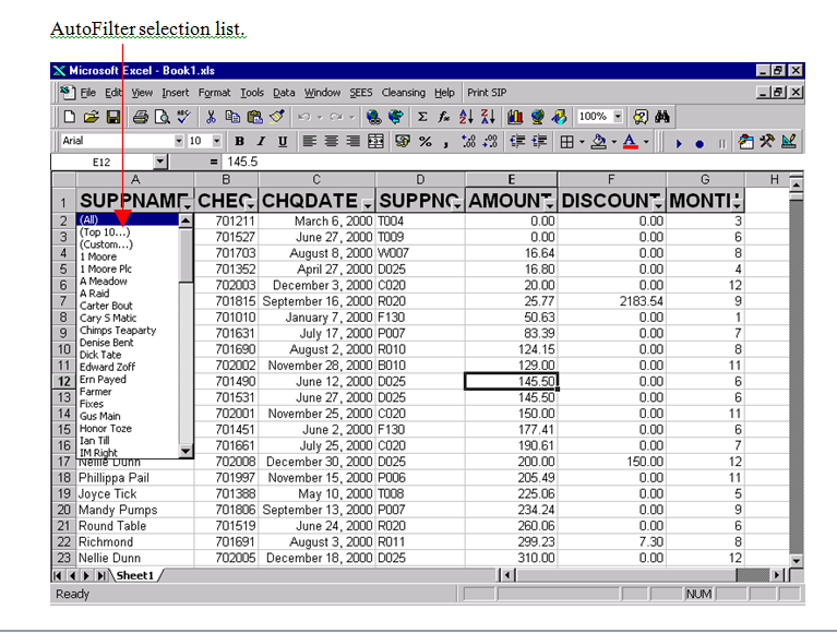
- Click on the data menu, click on the Filter command, and then click on the AutoFilter option.
- Click on the drop-down arrow next to the field name where you want to set criteria.
- Click on the set of criteria you want to view.
Custom Filtering Data
Using the AutoFilter is a very quick and easy way to find an exact match to criteria that you specify. Sometimes though you will need to find a range of answers rather than exact match, amounts between £3000 and £6000 for example, or names beginning with the letter B, for this you can use custom filtering.
To create a Custom AutoFilter
- Make sure that the AutoFilter command is switched on.
- Click on the drop-down arrow next to the field name where you want to set a custom filter.
- Click on the (Custom …) command.
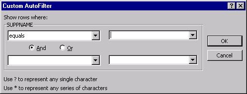
- The Custom AutoFilter dialogue box will be displayed.
- Under the Show rows where option, click on the box that contains the word equals.
- Type in the box to the right what you want to find, or click on the drop down arrow and choose from the list.
- Click on the And option if you want to set more than one criteria.
- When you have finished setting your criteria, click on the OK button.
Freezing Panes
Freezing panes is extremely useful when you have column or row headings which you want to keep in view when you scroll the screen to add more data.
To Freeze Panes
- Select the column to the right of the columns you want to freeze, or row beneath the rows to freeze.
- Click on the Window menu, and then click on the Freeze Panes command.
To Unfreeze Panes
- Click on the Window menu, and then click on the Unfreeze Panes command.
Download Sorting Data pdf :Autofilter and freeze panes
Other Lessons
- Introduction to Microsoft Excel
- Data Entry Auto Options
- Creating Formulae
- Formatting
- Introduction to charts
- Autofilter and Freeze panes
- Conditional Formatting and Comments
- Goal Seek and If Statements
- If Function And Or
- Give your Mouse a Brake in Excel


